Economics
The Post-Pandemic r*
The debate about the natural rate of interest, or r*, sometimes overlooks the point that there is an entire term structure of r* measures, with short-run…


The debate about the natural rate of interest, or r*, sometimes overlooks the point that there is an entire term structure of r* measures, with short-run estimates capturing current economic conditions and long-run estimates capturing more secular factors. The whole term structure of r* matters for policy: shorter run measures are relevant for gauging how restrictive or expansionary current policy is, while longer run measures are relevant when assessing terminal rates. This two-post series covers the evolution of both in the aftermath of the pandemic, with today’s post focusing especially on long-run measures and tomorrow’s post on short-run r*.
There is arguably some evidence that short-run r* is currently elevated relative to pre-COVID levels: The economy has proven to be extremely resilient and spreads remain relatively low, in spite of the recent banking turmoil. Estimates from the New York Fed DSGE model, which we discuss in tomorrow’s post, confirm this assessment. As shown in June, the model expects short-run real r* to be 2.5 percent by the end of the year. Evidence on whether long-run r*—that is, the persistent component, or trend, in r*—has risen after COVID is much weaker. We use a battery of models, from VARs to DSGEs, to estimate these trends, and these models reach different conclusions. According to VAR models, long-run r* has roughly remained constant and, if anything, declined a bit since late 2019, reaching 0.75 percent in real terms. According to the DSGE model, long-run r* has instead risen by almost 50 basis points during this period, and is now about 1.8 percent.
Long-Run r*: Different Answers from Different Models
The chart below shows the trends in r* obtained from two models presented in this Brookings paper by Del Negro, Giannone, Giannoni, and Tambalotti (2017). The two models are a “trendy” VAR (or, VAR with common trends; black dashed line) and a DSGE (blue dashed line) model capable of capturing low-frequency movements in productivity growth and the convenience yield. A key result of that paper, reproduced in the chart below with updated data, was that up to the mid-2010s these two very different methodologies delivered nearly identical results. After the pandemic, the estimates diverge notably however, with the VAR estimates trending down slightly, and the DSGE estimates trending up sharply.
The Low-Frequency Component of r* in the VAR and DSGE Models
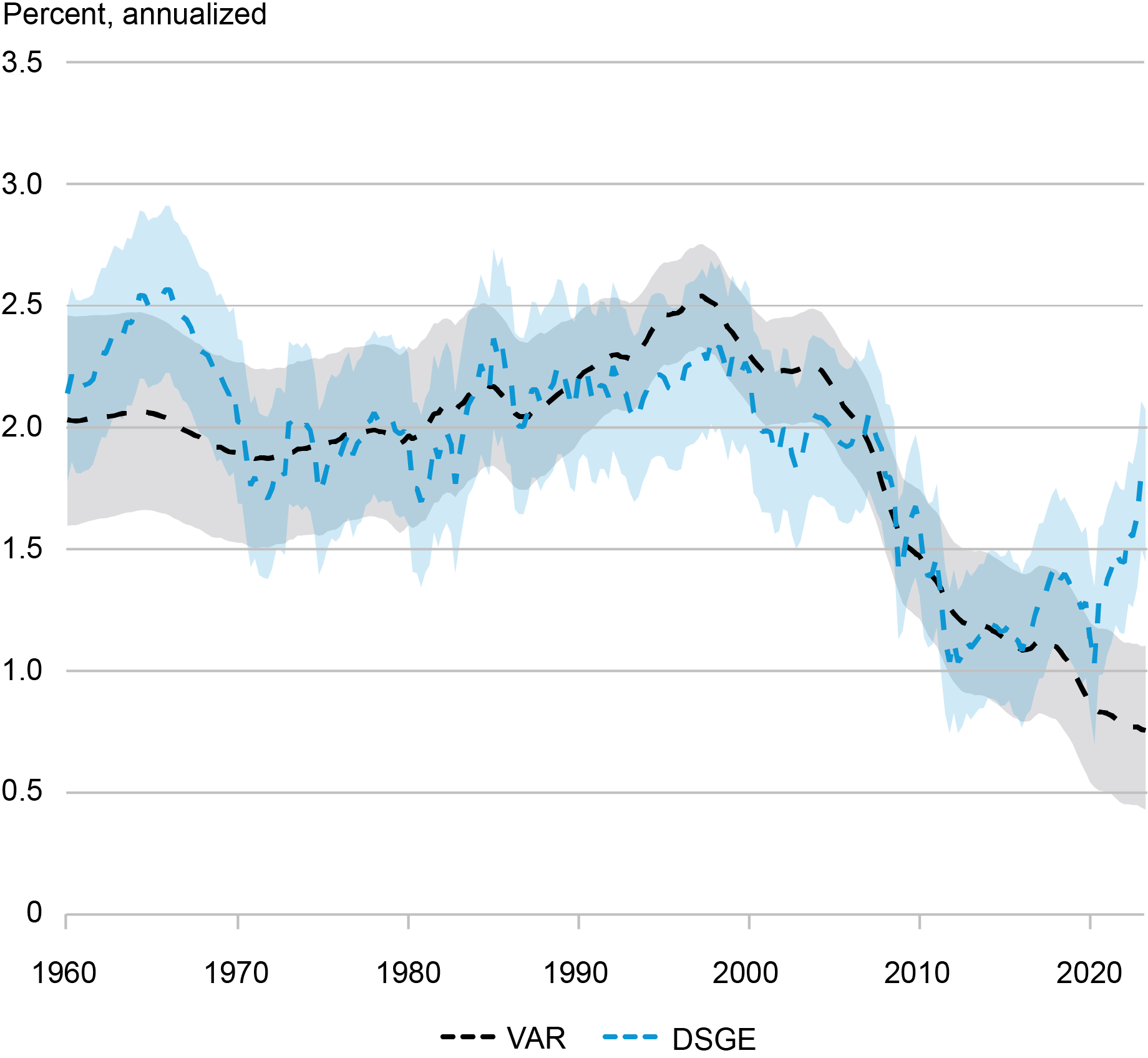
Note: The dashed black (blue) lines show the posterior medians and the shaded gray (blue) areas show the 68 percent posterior coverage intervals for the VAR (DSGE) estimates of the low-frequency component of the real natural rate of interest.
The table below reports numerical values of the changes in the r* trends (that is, long-run r*) according to a variety of models. It shows that from the fourth quarter of 2019 (pre-COVID) to the second quarter of 2023 the trend in r* has decreased by a little more than 10 basis points, according to the baseline trendy VAR. For a variant of this VAR where we also use data on consumption growth and hence make inference on trend growth, the decline is a bit larger at 20 basis points. According to the DSGE, long-run r* instead went up by almost 50 basis points after COVID. We also report the results from the global trendy VAR proposed by Del Negro, Giannone, Giannoni, and Tambalotti (2019). According to this model, which is estimated with annual data from seven advanced countries, both world and U.S. long-run r* rose by about 15 basis points from 2019 to 2022, although the increase is not significant.
The pre-COVID decline in long-run r* since the late 1990s is very similar to that reported in the Brookings paper, where the sample ends in 2016. According to the trendy VAR, long-run r* had fallen pre-COVID by a little more than 1.5 percentage points. The VAR with consumption implied a larger decline of almost 2 pp, while according to the DSGE the decline was about 1 pp. Because of the divergence in the post-COVID trends the overall decline in r* becomes a bit larger according to the two VAR models—1 and 1.75 pp, respectively—but falls to about 60 basis points according to the Brookings DSGE model.
Change in Long-Run r* According to Different Models
| Post-COVID Change 2023:Q2-2019:Q4 |
|||
| r*t | –cyt | gt | |
| VAR | -0.14 (-0.15, -0.12) Pr>0: 9 |
-0.06 (-0.09, -0.04) Pr>0: 20 |
|
| VAR with cons. | -0.19 (-0.22, -0.18) Pr>0: 7 |
-0.07 (-0.11, -0.05) Pr>0: 21 |
-0.10 (-0.13, -0.09) Pr>0: 16 |
| Brookings DSGE | 0.48 (0.06, 0.89) Pr>0: 98 |
0.28 (-0.01, 0.57) Pr>0: 96 |
0.20 (-0.04, 0.48) Pr>0: 94 |
| Global VAR | 0.14 (-0.44, 0.71) Pr>0: 68 |
||
| Pre-COVID Decline 2019:Q4–1988:Q1 |
|||
| r*t | –cyt | gt | |
| VAR | -1.61 (-1.78, -1.34) Pr<0: 99 |
-0.94 (-1.05, -0.89) Pr<0: 99 |
|
| VAR with cons. | -1.88 (-2.08, -1.52) Pr<0: 99 |
-0.73 (-0.83, 0.66) Pr<0: 99 |
-1.02 (-1.13, -0.86) Pr<0: 99 |
| Brookings DSGE | -1.03 (-1.51, -0.54) Pr<0: 99 |
-0.60 (-1.05, -0.14) Pr<0: 99 |
-0.39 (-0.62, -0.20) Pr<0: 99 |
| Global VAR | -1.69 (-3.27, -0.14) Pr<0: 98 |
||
| Post-COVID Decline 2023:Q2–1998:Q1 |
|||
| r*t | –cyt | gt | |
| VAR | -1.75 (-1.93, -1.46) Pr<0: 99 |
-1.01 (-1.13, -0.93) Pr<0: 99 |
|
| VAR with cons. | -2.07 (-2.30, -1.71) Pr<0: 99 |
-0.81 (-0.93, -0.71) Pr<0: 99 |
-1.12 (-1.26, -0.95) Pr<0: 99 |
| Brookings DSGE | -0.55 (-0.99, -0.24) Pr<0:99 |
-0.31 (-0.73, 0.09) Pr<0: 93 |
-0.19 (-0.44, 0.05) Pr<0: 94 |
| Global VAR | -1.56 (-3.17, 0.02) Pr<0: 97 |
Note: For each trend, the table reports the posterior median and the 95 percent (parentheses) posterior coverage intervals, as well as the posterior probability in percentage points that the change is positive (for the 2023:Q2-2019:Q4 period) or negative (for the 2019:Q4-1998:Q1 and 2023:Q2-1998:Q1 periods).
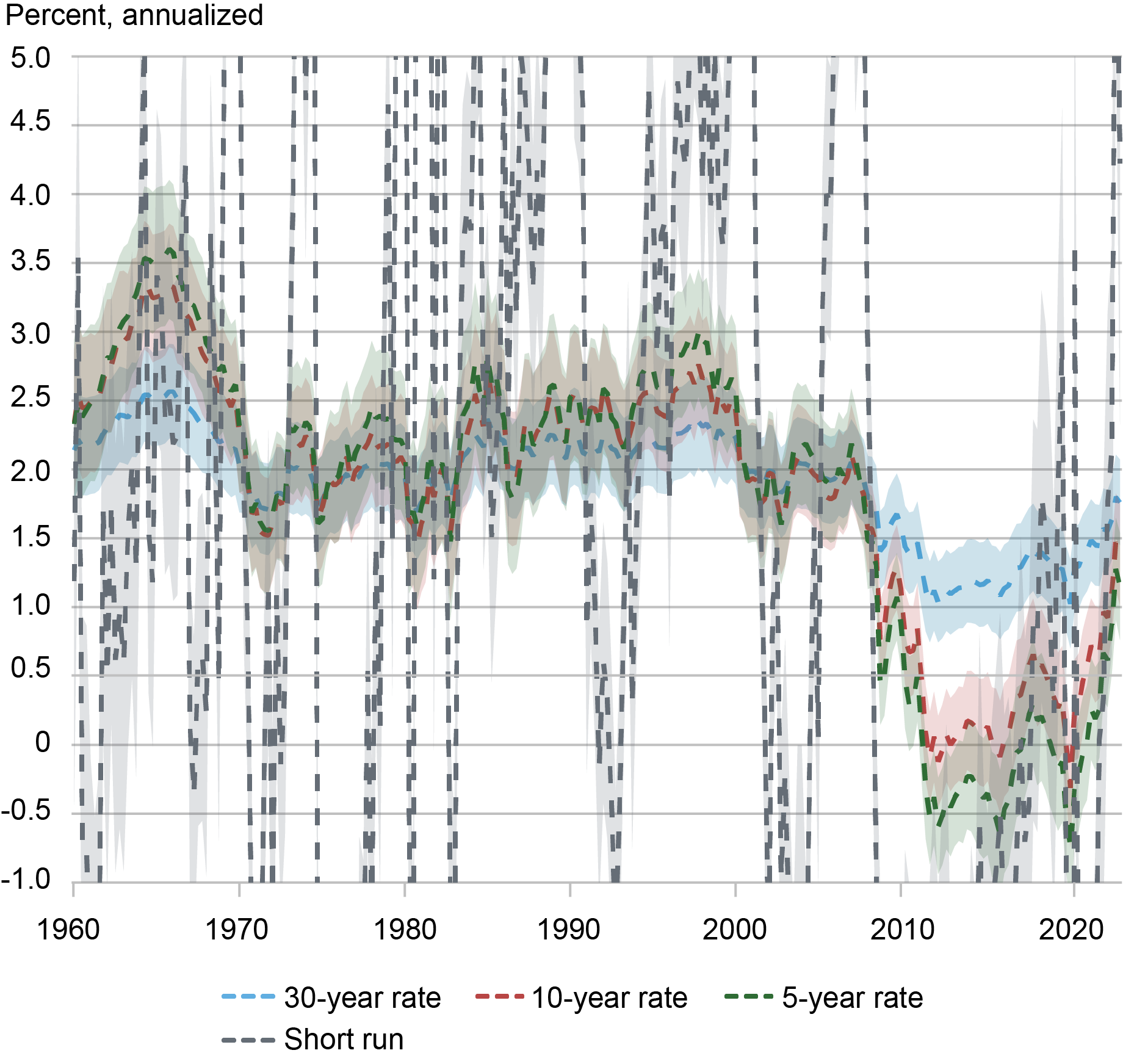
The Term Structure of r* in the DSGE Model
What drives these differences across models? Since much of the post-COVID action takes place in the DSGE model, we turn to this model in order to understand its interpretation of the data. The chart below shows the entire term structure of r* according to the model—namely the short-run r* and the 5-year, 10-year, and 30-year r* measures (which we have so far referred to as long-run r*), where the x-year r* is the expected value of r* x-years ahead (that is, the x-years r* is a forward rate). While the short-run r* is very volatile, its fluctuations capture well the state of the business cycle in the U.S.: short-run r* is low during recessions or periods of stagnation (for example, early 1990s, early 2000s, the great recession and its aftermath, and the COVID recession) and high when the economy is booming. Of late, the U.S. economy has remained extremely resilient even as monetary policy has tightened, as discussed in tomorrow’s post, and the estimates of r* are elevated.
The chart also shows that while the volatility of the r* measure not surprisingly diminishes with the horizon–5-year is less volatile than short-run r*, 10-year is less volatile than 5-year, and so on—all these measures are correlated with one another. This observation points to an important difference between trendy VAR and DSGE estimates of long run r*. While by design the trendy VAR separates the trend from the cycle—in econometric parlance, the model performs a trend/cycle decomposition—in the DSGE model all the various frequencies are inextricably linked. This does not mean that longer run DSGE measures of r* move with each and every movement of short-run r*—in the 1990s recession for instance short-run r* falls quite a bit but the other measures do not budge. However, it appears that in the DSGE, movements in short-run r* tend to have some information for longer run measures, while in the trendy VAR this information is ignored.
The Term Structure of r* in the DSGE Model
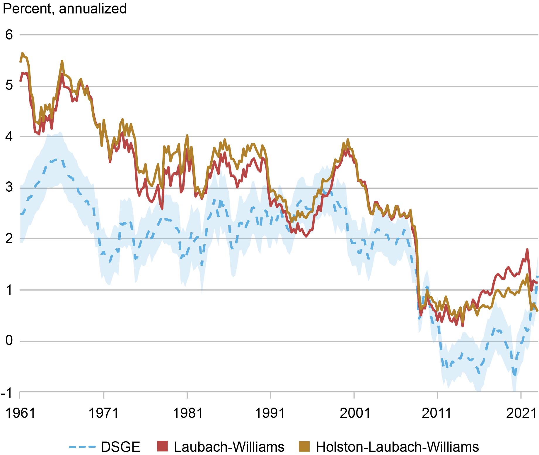
We conclude this post by relating the DSGE estimates to the r* estimates from Laubach and Williams (2003, LW) and Holston, Laubach, and Williams (2017, HLW), obtained with post-COVID data using the approach in Holston, Laubach, and Williams (2023). The chart below plots the time series of these measures together with the 5-year DSGE r*, which in the Brookings paper we found to be most correlated with the LW and HLW measures. The chart shows that the LW and HLW r* estimates declined sharply with the Great Recession, going from about 2.5 to 1 percent, after which they remain roughly steady at about 1 percent. The DSGE 5-year r* tracks the LW and HLW measures well from the early 1990s to the early 2010s. It then continues to decline going below zero, but eventually rises to a level comparable to that of the LW model at the end of the sample.
DSGE 5-Year r* and the LW and HLW Measures
Conducting inference on latent variables such as r* is a difficult business, as any estimate is inherently model dependent. In many circumstances the different models agree: for instance, there is widespread evidence that r* declined from the mid-1990s until the aftermath of the Great Recession and remained low until the COVID pandemic. Approaches disagree in terms of assessing what happened afterward, with models relying more on long-run averages indicating that long-run r* remained low, while approaches such as the DSGE where short- and long-run measures are more tightly connected indicate that long-run r* has risen. Tomorrow’s post focuses on short-run r* and its implications for the economy.
Katie Baker is a former senior research analyst in the Federal Reserve Bank of New York’s Research and Statistics Group.

Logan Casey is a senior research analyst in the Federal Reserve Bank of New York’s Research and Statistics Group.
Marco Del Negro is an economic research advisor in Macroeconomic and Monetary Studies in the Federal Reserve Bank of New York’s Research and Statistics Group.
Aidan Gleich is a former senior research analyst in the Federal Reserve Bank of New York’s Research and Statistics Group.

Ramya Nallamotu is a senior research analyst in the Federal Reserve Bank of New York’s Research and Statistics Group.
How to cite this post:
Katie Baker, Logan Casey, Marco Del Negro, Aidan Gleich, and Ramya Nallamotu, “The Post-Pandemic r*,” Federal Reserve Bank of New York Liberty Street Economics, August 9, 2023, https://libertystreeteconomics.newyorkfed.org/2023/08/the-post-pandemic-r/.


Disclaimer
The views expressed in this post are those of the author(s) and do not necessarily reflect the position of the Federal Reserve Bank of New York or the Federal Reserve System. Any errors or omissions are the responsibility of the author(s).
monetary
reserve
policy
fed
expansionary
monetary policy
stagnation


Argentina Is One of the Most Regulated Countries in the World
In the coming days and weeks, we can expect further, far‐reaching reform proposals that will go through the Argentine congress.

Crypto, Crude, & Crap Stocks Rally As Yield Curve Steepens, Rate-Cut Hopes Soar
Crypto, Crude, & Crap Stocks Rally As Yield Curve Steepens, Rate-Cut Hopes Soar
A weird week of macro data – strong jobless claims but…
Fed Pivot: A Blend of Confidence and Folly
Fed Pivot: Charting a New Course in Economic Strategy Dec 22, 2023 Introduction In the dynamic world of economics, the Federal Reserve, the central bank…